Graph theory, computed: every state on screen came from the algorithm

Twenty graph algorithms, computed once and drawn from the computation. BFS and DFS, Dijkstra and Bellman–Ford, Kruskal and Prim, Kahn's topological order, Kosaraju's components, Edmonds–Karp with its min cut, greedy colouring, Kuhn's matching with König's cover, Hierholzer's Euler circuit, low-link connectivity, and — since 0.8.0 — Prüfer codes, Jordan centres, ear decompositions, Gale–Shapley, Hamiltonian search, edge colouring and degeneracy orderings live in one module, straightedge/graphs.py. The Manim scene and the SVG storyboard both read its step trace, so a video and a handout of the same request cannot disagree about which vertex was settled third — and neither can show a state the algorithm did not reach.

The trace is a list of roles, not colours: this vertex is current, these are the frontier, that edge is in the tree, this one was rejected. Each lane maps roles onto its own palette. What a step also carries is the thing a lecture writes on the board beside the graph — the queue, the distance table, the running forest weight — and a caption, which is the sentence the narration should say over it. One step, one narration beat: the video's whole structure is the algorithm's.

Computed once, drawn twice

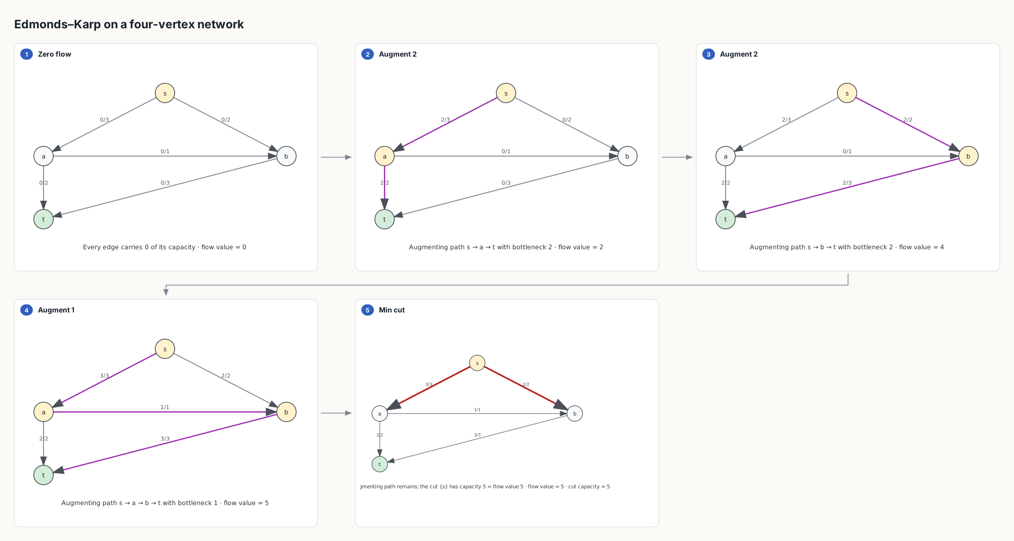
Five panels of Edmonds–Karp on a four-vertex network: three augmenting paths highlighted in turn with flow/capacity labels updating, then the min cut with the source side shaded and the caption stating that the cut capacity equals the flow value, 5. — The same algorithm as a printable storyboard — `graph_algorithm` with `animate: false`. Video and storyboard read one step trace, so the fourth panel here is the fourth beat of a video of this network; nothing is re-derived on the way to the page.

Refused, with the witness

The half of this that matters for a lab is what happens when the graph makes the request false. Ask for a topological order of a graph with a cycle and no drawing tool will stop you; most will happily number the vertices. Here the algorithm raises, and what it raises carries the structure that proves it:

$ straightedge draw graph_algorithm --params '{"algorithm": "topological_sort",
    "directed": true, "nodes": [{"id":"A"},{"id":"B"},{"id":"C"},{"id":"D"}],
    "edges": [{"from":"A","to":"B"},{"from":"B","to":"C"},{"from":"C","to":"A"},{"from":"C","to":"D"}]}'
'graph_algorithm' was refused: the graph has a cycle, so it has no topological order: A → B → C → A

The same gate runs before a video. Dijkstra is handed a negative weight and the precondition says so, in the algorithm's own terms, before Manim is asked for a single frame:

$ straightedge scaffold --template graph/shortest_path \
    --params '{"algorithm": "dijkstra", "nodes": [{"id":"A"},{"id":"B"}],
               "edges": [{"from":"A","to":"B","weight":-2}]}'
[error] graph/shortest_path: edge 'A'–'B' has negative weight -2; Dijkstra requires
        nonnegative weights; nothing would be drawn
1 precondition(s) say this plan will not show what was requested.

Bellman–Ford accepts that weight and refuses a negative cycle instead — B → C → B, vertex by vertex. An Euler circuit on K₄ is refused with the four odd-degree vertices. A matching is refused if an edge sits inside one side of the declared partition. Each of these is the exercise's actual content: the reason there is no answer is the answer, and it arrives as a named structure a student can check by hand, not as a blank canvas or a plausible picture of something that is not so.

The edges Kruskal refuses

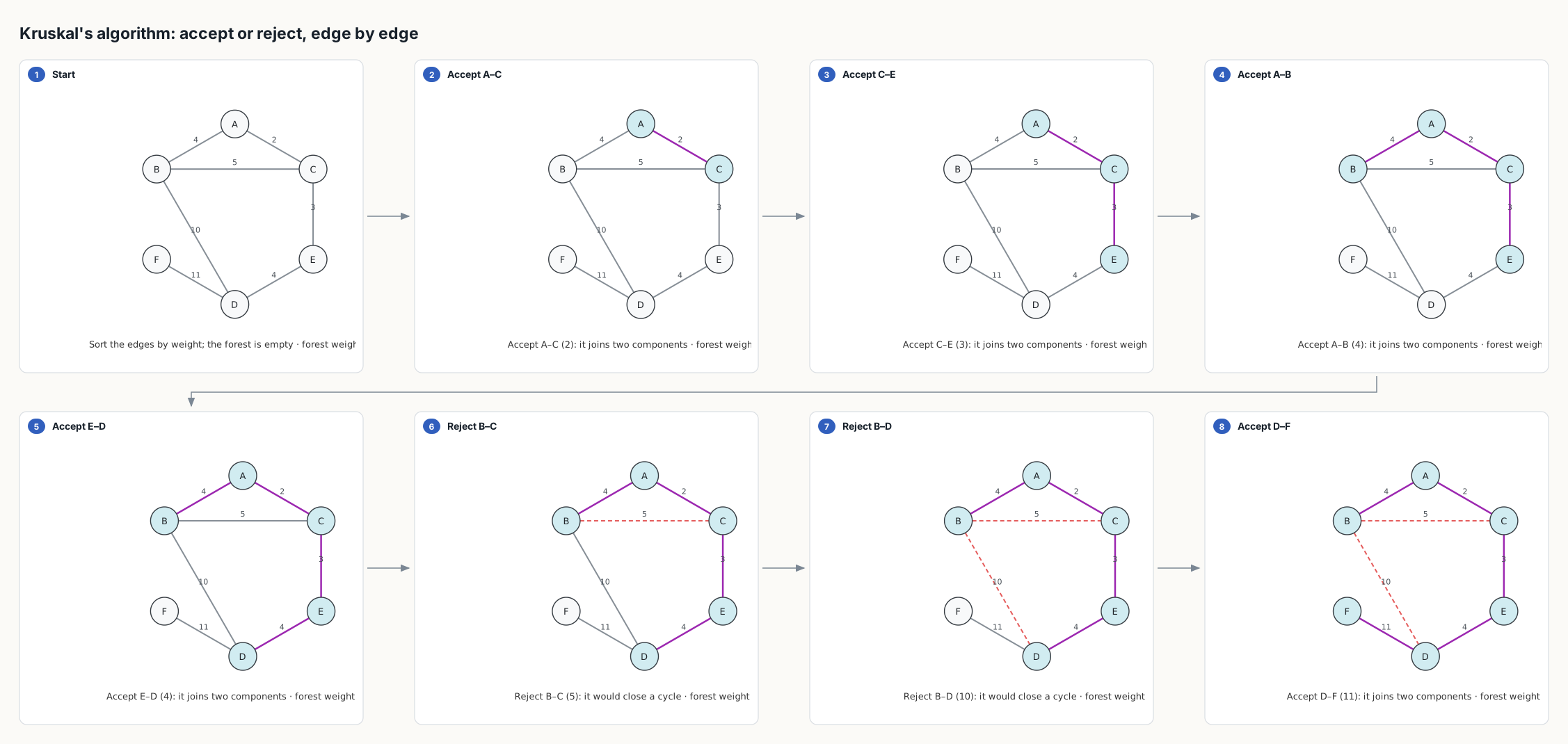
The same graph as an SVG storyboard, no Manim involved. The two edges Kruskal rejects are drawn dashed rather than left out — the rejection is the lesson, and a storyboard that silently skipped B–C would be teaching the wrong algorithm.

Prim, run on the same graph, ends on the same tree and the same weight, 24 — which the test suite asserts rather than trusts. Every algorithm here is checked against a property a textbook states: Prim and Kruskal agree; the max flow equals the cut it ends on; König's cover has exactly the matching's size; DFS agrees with the recursive reference on graphs with cross edges, which is precisely where the usual iterative-stack shortcut draws a "DFS tree" no depth-first search produces.

Without Manim, without JavaScript

A wheel graph on six vertices being greedily coloured, one vertex per frame, each frame cross-fading into the next; the hub takes a fourth colour. — Greedy colouring of a wheel as a native animated SVG: the frames are the computed states, cross-faded with SVG's own timing. It plays in any browser, in a slide, in a wiki — and a client that asks for reduced motion sees the first frame, still.

What each one needs, and what it refuses

Algorithm	Needs	Refused with
BFS · DFS	a start vertex	—
Dijkstra	weights ≥ 0	the negative edge
Bellman–Ford	weights	the negative cycle
Kruskal · Prim	undirected, weights	—
Topological sort	directed	the cycle
Strongly connected components	directed	—
Max flow · min cut	directed, capacities, s ≠ t	s = t, an uncapacitated arc
Greedy colouring	—	—
Bipartite matching · König cover	a declared partition	an edge inside one side
Euler circuit / trail	connected edges	the odd-degree vertices
Bridges · articulation vertices · blocks	undirected	a directed graph
Prüfer encode · decode	a tree, or a code	the cycle, the first differing code position
Tree centre	a tree	the cycle or the components
Ear decomposition	2-connected	the articulation vertex
Stable matching	complete strict preferences	the blocking pair
Hamiltonian search	a start, a frame budget	the found cycle, or the exhausted search
Edge colouring	—	the vertex two same-class edges share
Degeneracy ordering	—	—

All twenty are in the SVG lane as graph_algorithm. Five concepts — traversal, shortest path, spanning tree, max flow, connectivity — are also Manim videos under the graph topic, reachable by prompt on a stock graph or by template with your own.

Four constructions a course draws often enough to earn their own template are checked the same way. turan builds T(n,r) and reports the verified edge count; mycielski builds the shadow layer and hub over your base graph, colours it, and confirms it stayed triangle-free; floyd_warshall shows one distance table per intermediate vertex and refuses a negative cycle with the cycle; havel_hakimi reduces a degree sequence step by step and realises the graph on the way back up, or stops at the entry that went negative.

The structures a graph lesson keeps beside the graph are computed the same way. block_cut_tree derives the blocks and the articulation vertices that join them from the low-link pass; disjoint_set runs union by rank with path compression and refuses a find whose expected root is wrong; priority_queue executes insert, decrease-key and pop-min on a binary heap and refuses a claimed minimum that is not the minimum; graph_representation draws one graph next to its adjacency list, adjacency matrix and incidence matrix so the three cannot disagree.

Run it on your graph

git clone https://github.com/SciMigo/straightedge
cd straightedge && python3 -m pip install -e '.[render]'

# a video of Dijkstra on your graph — one narration beat per computed step
straightedge render --template graph/shortest_path --params '{
  "algorithm": "dijkstra", "start": "A",
  "nodes": [{"id":"A"},{"id":"B"},{"id":"C"},{"id":"D"}],
  "edges": [{"from":"A","to":"B","weight":2},{"from":"A","to":"C","weight":5},
            {"from":"B","to":"C","weight":1},{"from":"B","to":"D","weight":4},
            {"from":"C","to":"D","weight":1}]}'

# the same states as a printable storyboard, no Manim needed
straightedge draw graph_algorithm --params '{"algorithm": "dijkstra", "animate": false, ...}'

A frame is at most eight vertices and seventeen beats; past that a video stops being one lesson and becomes a log, and the precondition says so instead of rendering it small. The SVG storyboard holds twelve panels and the animated SVG twenty-four frames, on the same principle.

What this is for

A lab. The student brings the graph — an edge list, a homework figure — and the question is not "what does Dijkstra look like" but "is my table right, and if not, where does it first go wrong". Because every state is computed, the answer is a step number and a caption. Because a false claim is refused with its witness, "there is no topological order" comes back as the cycle, and "this is not bipartite" as the odd cycle. The picture is the last thing produced, and it is produced from the run.

The picture cannot show a state the algorithm did not reach